Navigation:  Sample Session > Entering Data

Below is a diagram for a wood roof beam we wish to design.

 

 

 

The following steps will guide you through the process of setting the span lengths and entering the loads as shown. (In a subsequent step we will select the member section size and reference design values from the internal databases.)

 

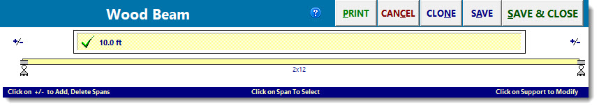
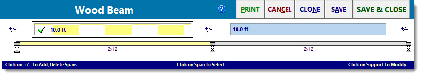
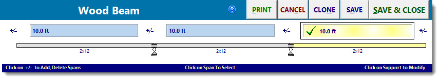
The top portion of the screen should currently look like this:

 

 

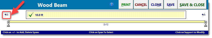
The first thing we will do is add the left cantilever.  To do this, click the [+/-] icon at the left end of the beam as shown bubbled below:

 

 

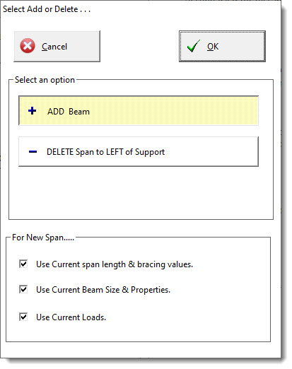
This opens the dialog named Select Add or Delete. It is currently set up to allow us to add a new beam span, which is exactly what we want to do. There are some additional settings offered at the bottom of the dialog in the form of checkboxes.  We don't need to worry about these at this point, but it's good to know that they are available, because they can offer some time-saving conveniences in certain modeling situations.

 

See the image of the Select Add or Delete dialog shown below:

 

 

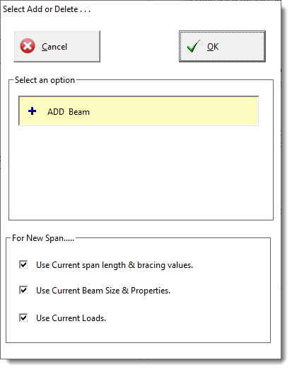
For our purposes, all we need to do is click the [OK] button. This inserts a new beam span to the left of the original beam as shown below:

 

 

At this point, don't be concerned about the fact that the new span is not a cantilever and that it is not the intended length.  We'll correct both of those items in just a moment.  For now, let's repeat a similar process to add a new beam span on the right.  First click the [+/-] icon that appears above the right-most support. The following dialog appears:

 

 

This is very similar to the Select Add or Delete dialog we saw before, except that it now has an extra option to delete the span that is to the left of the support.  Although we don't want to do this, it's good to know that this is the way that you would delete a span if necessary. What we want to do is add a new beam span, and that is the option that is currently selected (highlighted in yellow), so we can just click the [OK] button.

 

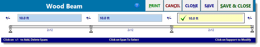
The screen should now display a 3-span continuous beam as shown below:

 

 

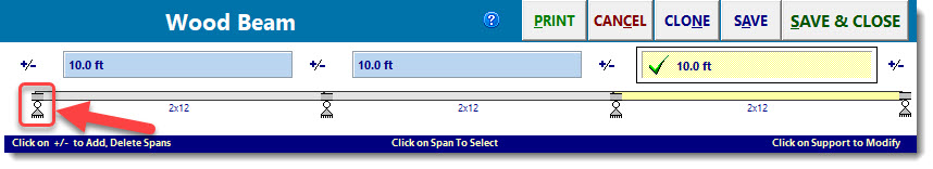
Now that we have three spans to work with, let's modify the support conditions to create the cantilevered spans at the left and the right. To do this, click on the left-most support icon shown bubbled below:

 

 

This will open the following pop-up menu that offers many options for defining the support condition at that location:

 

 

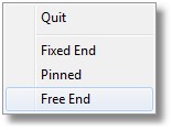
Click the Free End option to remove all restraint from the left end, creating a cantilever. Repeat the same process at the right-most support, but leave the remaining two supports as they are currently configured.  (They represent pinned conditions that prevent translation in all directions but offer no moment restraint.) The result will be the double-cantilevered beam as shown below:

 

 

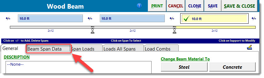
Now that the support conditions have been established correctly, we can wrap up this exercise by modifying the span lengths to match the problem definition. Start by clicking the Beam Span Data tab shown bubbled below:

 

 

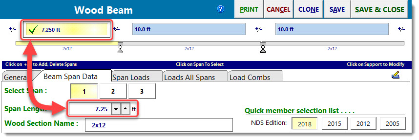
The screen layout will change to display the Beam Span Data tab as shown below:

 

 

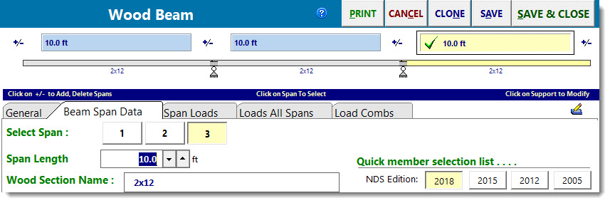
Now, we just need to adjust the span lengths for each of the three spans.  

 

First, note that the graphical depiction of the beam helps us to make the association between the three individual spans and the span numbers.  Click any of the three span number buttons in the Select Span area and notice that a corresponding span becomes highlighted in the large graphic at the top of the view.  Using this method, we can confirm that the spans are logically ordered from number one on the left to number three on the right. (Note that you can also click the highlighted rectangles shown above each beam span, and they act in exactly the same way that the numbered buttons do.)

 

So to finish things off, click the button for span [1] and verify that the left span becomes highlighted. According to the problem statement, this span is supposed to be 7'-3", so you can highlight the value that is presently displayed in the Span Length field, manually edit it to say 7.25, and then press the [Tab] key to enter that value. The display will update to show the proper span length for the left beam span as shown below:

 

 

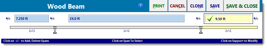
Repeat the same process to set the Span Length for the middle span to 24'-0" and to set the Span Length for the right span to 9'-6", at which time the display should appear as shown below:

 

 

The next step will be to enter the loads on the beam. Let's begin by entering the concentrated load at the free end of the left beam span. Click the Span Loads tab to display the following screen:

 

 

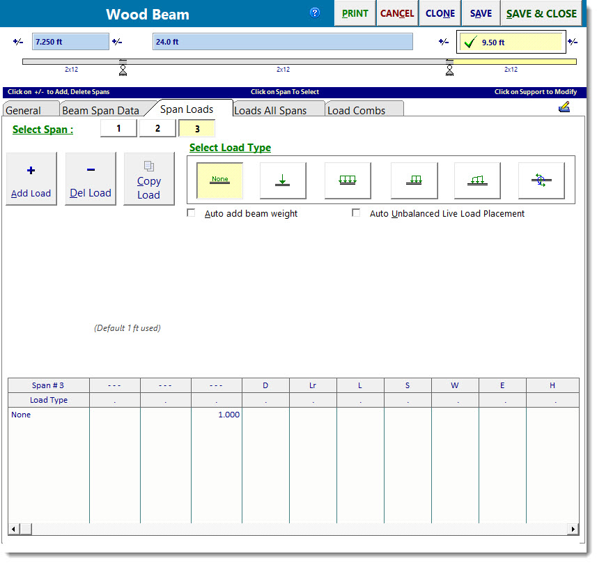
This screen contains tools to apply loads to a selected span at a time.  (Shortly, we will see a convenience tool that will allow us to apply loads to ALL spans of a beam at one time.)

 

Since we want to start by entering the concentrated load at the free end of the left beam span, click the [1] button in the Select Span area to put the focus on Span 1.

 

The blue highlighted band in the table now represents the first load on Span 1. But it currently indicates Load Type = None, because we have not defined the load yet. Click the button indicated in the screen capture below to identify the load as being a concentrated load:

 

 

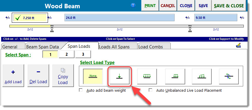
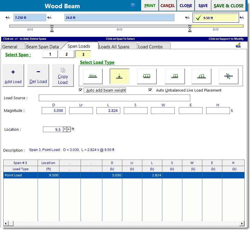
This will reconfigure the screen with the appropriate input fields to fully define the magnitude, direction, and location of the concentrated load as shown below:

 

 

 

Select the checkbox for the Auto add beam weight option.  This will trigger the program to determine the self weight of the beam that we eventually choose, and apply it as dead load when the analysis is performed.

 

Select the checkbox for the Auto Unbalanced Live load Placement option. This will initiate the generation of additional loading conditions to ensure that all possible permutations of live load placement are properly examined. Note that selecting this option can lead to longer analysis times because of the number of different conditions that must be analyzed. However, with the double-cantilevered beam configuration, it would be important for us to have the module examine all of these potential loading permutations.

 

The Load Source input field provides a location where you can add some descriptive text for your own use to identify this particular load item. The use of this field is optional, so for this sample session we will leave it blank.

 

When defining the magnitude of the concentrated load, note that the module is set up to receive this kind of load in units of kips, and notice that it has input fields for the common load cases, such as Dead, Live, Snow, etc.

 

Click in the input field for Dead, enter a magnitude of 3.03, and then press the [Tab] key. This enters the Dead load magnitude and moves the cursor to the next input field.

 

Note: For convenience this module is configured such that loads with positive magnitudes are assumed to act downward, since the majority of the load items are typically gravity loads of some sort.

 

The cursor is currently in the Lr input field, which represents Roof Live load.  We don't need to enter any magnitude for Roof Live, so press the [Tab] key once again to place the cursor on the Live load input field. Enter a magnitude of 2.824, and then press the [Tab] key.

 

The final step in specifying this concentrated load is to identify its position using the Location input field. Always specify the distance from the left end of this span to the position of the concentrated load. In this case, the correct value is zero, which also happens to be the default value for the Location field, so the Location field can be left as-is.

 

The screen should now appear as shown below:

 

 

The next step will be to define the other concentrated load, which occurs at the free end of the cantilever on the right end of the beam, by following a very similar process.

 

Click the [3] button in the Select Span area to put the focus on Span 3.

 

Click the button to identify the load as being a concentrated load.

 

The magnitudes of this load are the same as those used at the opposite end of the beam, so click in the input field for Dead, enter a magnitude of 3.03, and then press the [Tab] key twice.  

 

In the Live load input field enter a magnitude of 2.824, and then press the [Tab] key.

 

This concentrated load is to be positioned at the extreme right end of this span, so click in the Location input field, enter a distance of 9.5 (9'-6" from the support at the left end of Span 3), and then press the [Tab] key. The screen should now appear as shown below:

 

 

The next step in defining loads is to apply the uniformly distributed load across all three spans. This could be done by using the Uniformly Distributed Loading Type here on the Span Loads tab. But this would require some repetition, because the Span Loads tab is specifically set up to facilitate the application of loads to one span at a time.

 

To apply this load in a more efficient manner, click the Loads All Spans tab shown bubbled below:

 

 

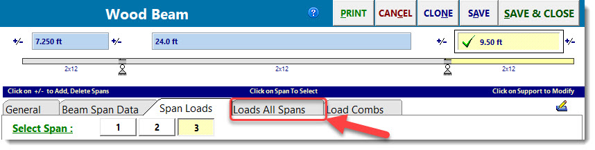
The screen will reconfigure itself to display different tools for applying various types of loads to all spans of the beam. The one that is most appropriate for our application is the one shown bubbled below:

 

 

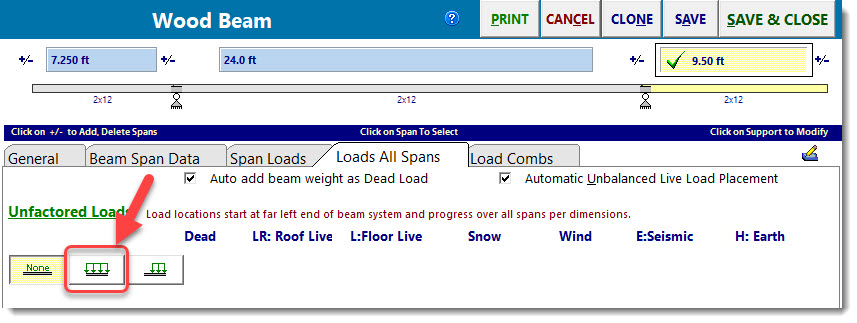
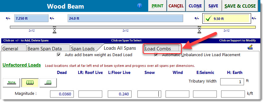
Click that tool and note that the screen displays input fields for Tributary Width and load magnitudes for the various Load Cases as shown below:

 

 

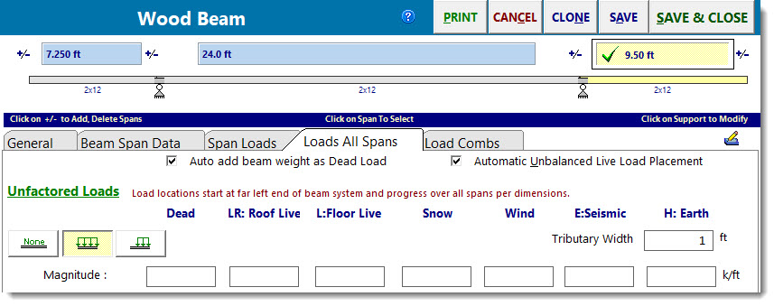
Note: When using this tool, you can either leave the Tributary Width input field at its default value of 1.0, and then enter the magnitudes for the various load cases in units of kips per foot, or you can specify a Tributary Width magnitude other than 1.0 foot, and then enter the magnitudes for the various load cases in units of kips per square foot, which will be multiplied by the Tributary Width to determine the magnitude of the effective line load in units of kips per foot.

 

For the purposes of our exercise, we will leave the Tributary Width input field at its default value of 1.0.

 

Click in the Dead load input field, enter a magnitude of 0.036, and press the [Tab] key twice.

 

In the Live load input field, enter a magnitude of 0.24, and press the [Tab] key once more.

 

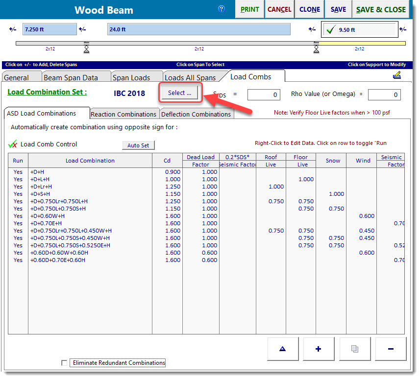
The last item to take care of is to observe the load combinations that will be used for design. Click the Load Combinations tab indicated below:

 

 

This will display the Load Combinations screen. On this screen, you can select the desired Load Combination set.  In this case, we are already referencing the IBC 2018 load combinations, which is our goal.  But if that selection did need to be changed, click the "Select" button indicated in the screen capture below:

 

 

This will open a pop-up menu offering choices of load combination sets that exist on the current machine, similar to the one shown below:

 

 

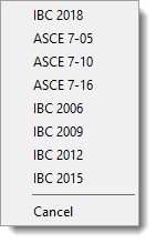
Choose the option named IBC 2018.  This will set up the calculation to use load combinations based on IBC 2018.

 

Next, click the button, and confirm by clicking the [Yes] button. This is a very convenient option for wood designs, because it automatically sets the CD value based on the shortest duration load case within each load combination. Note the various values of CD that result.

 

The final step in this section is to ensure that all of the listed load combinations will be used in the analysis and design. To do this, click the Load Combination Control button button. This will open a pop-up menu offering options for marking and clearing the Run status of all of the load combinations in the list, as shown below:

 

 

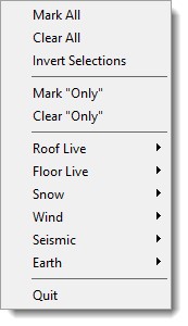
Simply click the [Mark All] option, and all of the load combinations in the list will be marked for use in the analysis and design.