Loads |
  
|
Loads |
|
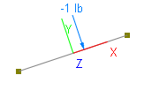
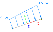
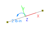
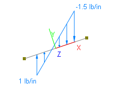
Point loads or line loads may be applied to a member. Point loads may be forces or moments. Line loads must be forces. You may specify loads in either the global or local coordinate system. The locations of loads must be in ratios of the member length, measured from the start of the member. The following figure shows examples of point and line loads.
Point Loads |
Line Loads |
|---|---|
local y force, distance=0.6 |
local y force, start distance=0,end distance=1 |
local z moment, distance=0.4 |
global Y force, stat distance=0.2, end distance=0.8 |
The self weight of members may be calculated automatically if the material weight densities and self weight multiplier are nonzero. By default, self weight acts in the negative global Y direction. You may however change the direction to positive or negative direction of the global X, Y, or Z. This flexibility is useful in some circumstances. For example, if you model a grillage on the XY plane, the self weight may be either in the positive or negative global Z direction, depending on your preference on load sign convention. To activate automatic self weight calculation, use the command Loads > Assign Self Weights.
An area load may be applied to multiple members on a whole planar area. The area is defined by three or four coplanar nodes. The area load is then distributed as line loads to perimeter members of enclosed sub-areas within the load area prior to static or dynamic solution. Area loads are distributed to perimeter members that form each of the enclosed sub-areas according to the following methods:
-Two-way (rectangular sub-areas)
-Short-Sides (rectangular sub-areas)
-Long-Sides (rectangular sub-areas)
-AB-CD Sides (rectangular sub-areas)
-BC-AD Sides (rectangular sub-areas)
-Centroid-based
-Circumference-based
The first five distribution methods apply to four-node rectangular sub-areas only. The centroid-based method may be applied to convex sub-areas only. The circumference-based method may be applied to both convex and concave sub-areas. Loads may also be distributed to sides parallel to AB-CD or BC-AD sides of the load area. The program is intelligent enough to determine the most appropriate load distribution if inconsistencies arises. For example, if you select two-way distribution method for a sub-area that is not rectangular, the program will use the centroid-based method if the sub-area is convex or the circumference-based method if the sub-area is concave.
The program allows you to convert area loads to line loads directly and automatically. This feature allows you to see how exactly the program would distribute area loads to members prior to the solution. Of course, you can always undo the conversion if you want to keep the area loads. For more information on the load conversion, please see Loads > Assign Area Loads.
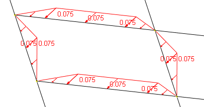
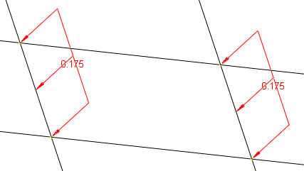
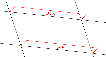
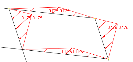
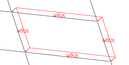
As an example, let’s say we have a 3.5 x 1.5 ft rectangular sub-area subjected to 100 lb/ft^2. The following line loads are converted from the same area load based on different distribution methods.
Two-way Distribution |
|---|
Short-side Distribution |
Long-side Distribution |
Centroid-based Distribution |
Circumference-based Distribution |
Area loads may be specified in either the local or global coordinate system. Global area loads may be in the global X, Y, or Z direction. Local area loads may only be in the local z direction, which is perpendicular to the load area. It is recommended that area loads be defined in their own load cases. In this way, you will find it easier to identify, edit, and delete area loads later on.
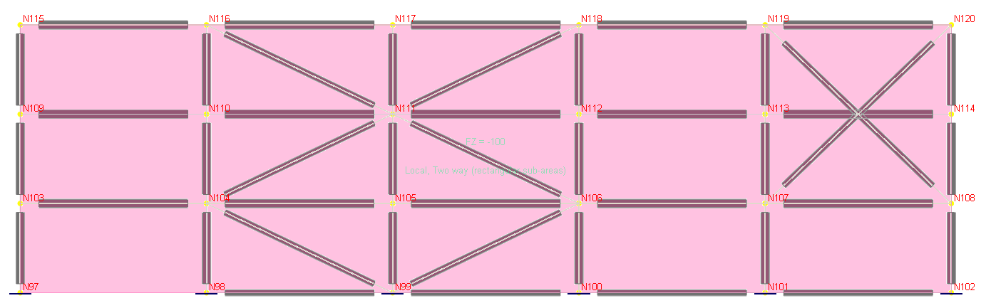
There are a few limitations to the area load concept in the program. The first limitation is that the sub-areas must be close-formed by perimeter members. In the following figure, the sub-area formed by node 97, 98, 104 and 103 is not a closed sub-area because there is no member connecting the node 97 and 98. As a result, no area loading will be distributed to the three perimeter members from the sub-area. The second limitation is that sub-areas must not overlap. In Figure 16.3, the sub-areas in node 101, 102, 120 and 119 are overlapping. This will result more load being distributed to the members in these sub-areas. The program gives a warning when the area load footprint is not equal to the total actual loaded area. The problem may be solved by splitting members 119-108, 107-120 and 113-114 at the intersection point.
The third limitation is that any sub-area may not contain more than one concave node (with internal angle more than 180 degrees). The fourth limitation is that any sub-area may not contain the same node more than once in forming the perimeter polygon.
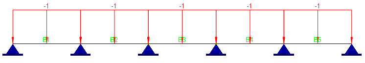
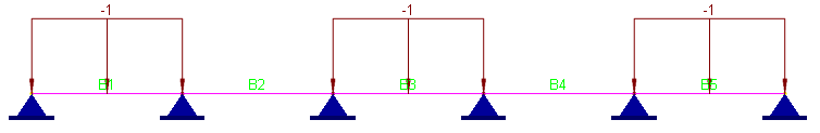
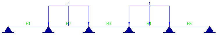
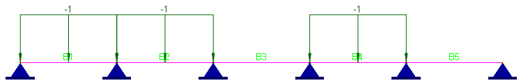
The program offers automatic generation of live load patterning (point and line loads only). The following figure shows how the program generates load patterning on a five-span continuous beam. Loads on each generated pattern reside in a separate load case automatically generated. Additional load combinations are generated as needed as well.
All Spans |
|---|
Odd Spans |
Even Spans |
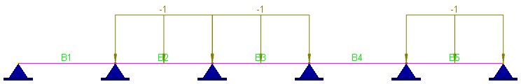
Second Support + Alternate Spans |
Third Support + Alternate Spans |
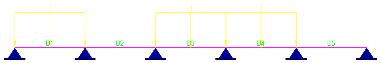
Fourth Support + Alternate Spans |
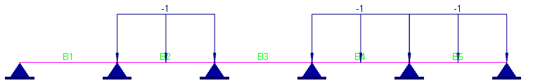
Fifth Support + Alternate Spans |
The program also offers automatic generation of moving loads (point loads only). The mechanism employed by the program is similar to the live load patterning.
 <
<