Navigation:  Calculation Modules > Analysis > ENERCALC 3D > Ribbons > Analysis > Analysis Options

Analysis > Analysis Options prompts you with the following dialog.  

 

 

 

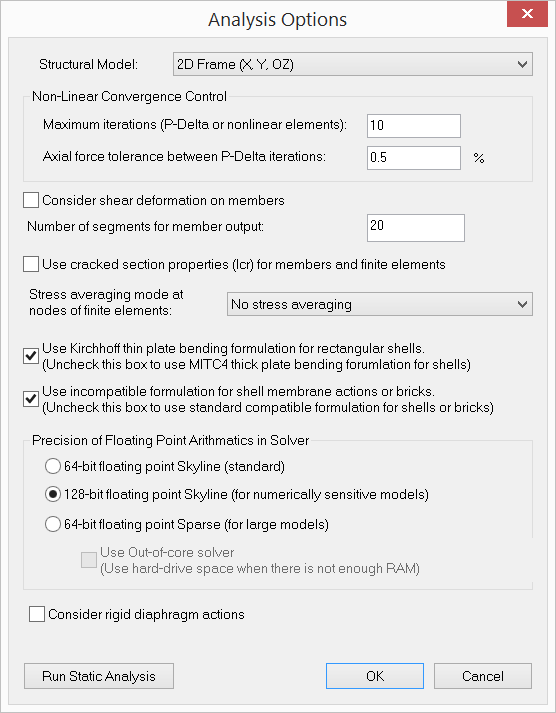
It allows you to set important options before performing analysis on the model.  

 

The “Model type” determines the type of the model to analyze.  Model type “3D Frame & Shell” is the most general.  It has all six degrees of freedom (DOFs) available to every node in the model.  Any model may be analyzed with this model type.  However, computer memory or time may be wasted if a simpler model can be used.

 

Model type “2D Frame” may be used to model a 2D frame (beams and trusses) structure in the XY plane.  Only three DOFs (Dx, Dy and Doz) are available to every node in the model.  The rest of the DOFs are suppressed.  

 

Model type “3D Truss” may be used to model 3D truss structures.  Only three DOFs (Dx, Dy, and Dz) are available to every node in the model.  The rest of the DOFs are suppressed.  If the model contains both 3D trusses and beams, “3D Frame & Shell” model type must be used and appropriate moment releases assigned.

 

Model type “2D Truss” may be used to model 2D truss structures in the XY plane.  Only two DOFs (Dx and Dy) are available to every node in the model.  The rest of the DOFs are suppressed.  If the model contains both 2D trusses and beams, “2D Frame” model type must be used and appropriate moment releases assigned.

 

Model type “2D Plate Bending” may be used to model 2D plate bending structures such as flat slabs or mat foundations in the XY plane.  It uses only the plate bending action of the shell formulation.  Only three DOFs (Dz, Dox and Doy) are available to every node in the model.  The rest of the DOFs are suppressed.  The self weight should be in either –Z or +Z direction depending on your sign convention for loads.

 

Model type “2D Plane Stress” may be used to model 2D plane stress structures such as shear walls in the XY plane.  It uses only the membrane action of the shell formulation.  Only two DOFs (Dx and Dy) are available to every node in the model.  The rest of the DOFs are suppressed.

 

Model type “3D Brick” may be used to model 3D solid structures.  Only three DOFs (Dx, Dy, Dz) are available to every node in the model.  The rest of the DOFs are suppressed.

 

Non-linear convergence control includes the maximum iterations and axial force tolerance between adjacent P-Delta iterations.  The maximum iterations apply to both P-Delta analysis and analysis involving non-linear springs.  It is provided to avoid excessive number of nonlinear iterations during the solution.  A default value of 10 is usually sufficient.  Axial force tolerance between adjacent P-Delta iterations reflects the actual convergence of the P-Delta analysis. The default value of 0.5% should be good for most cases.  It is a good idea to perform a linear analysis before the P-Delta analysis.  In this way, you may identify any problems in the model before the more rigorous analysis option is undertaken.

 

By default, the program considers shear deformations on members in the model.  You must also set shear areas of member sections for this option to take effect.  To do that, click Create (or Modify) > Member Properties > Member Sections.  You may ignore member shear deformations by unchecking “Consider shear deformation on members”.  Generally, shear deformations on members are insignificant.  However, you should check this option when members are of relatively great depths. Shear deformation, when considered, applies to both the element stiffness matrix and local (segmental) deflections.

 

The number of segments for member segmental output may be set from 1 to 127.  A value of 20 segments is recommended in most cases.  More segments produce more accurate results, but require more usage of computer memory.  The accuracy may be reflected in the smoothness of moment, shear and deflection diagrams.  Since member local deflection is computed based on the moment and shear diagrams, a value of more than 20 segments may be needed if very accurate local deflection is desired.

 

You may specify whether to use cracked section properties for the analysis.  The cracking factors are specified in Create (or Modify) > Member Properties > Cracking Factors or Concrete Design > Cracking Factors.  Cracking factors will not be applied until “Use cracked section properties (Icr) for members and finite elements” is checked here.  This option is given so that you do not need to reenter cracking factors if you decide to use gross section properties in a different analysis run.

 

Usually, stresses in finite elements are not continuous across element boundary.  You may average them for adjacent shells/bricks at nodes.  This usually makes the results more accurate and the contours smoother.  However, it may also disguise insufficient convergence for an unsatisfactory (coarse) finite element mesh. Obviously, stress averaging can only apply to adjacent elements that have compatible local coordinate systems.  For planar elements, stress averaging should only apply to adjacent elements that share the same local coordinate systems.  Special attention should be given to shear stress averaging at supports since shears of adjacent elements may have opposite signs.

 

By default, the program uses the MITC4 for shell bending formulation.  The MITC4 is a thick plate formulation and accounts for the out-of-plane shear deformation.  However, if the shell elements are all rectangular, you may use the classical Kirchhoff plate bending formulation.  The Kirchhoff plate element is a thin plate formulation and ignores the out-of-plane shear deformation.

 

For the membrane formulation of the shell element or of the brick element, incompatible modes may be added to the standard isoparametric (compatible) formulation.  The incompatible shell element models the in-plane bending more accurately than the standard compatible element.  The incompatible brick element, which produces much more accurate results than the compatible one, should almost always be preferred.

 

There are three kinds of solvers available in ENERCALC 3D:

 

Double precision 64-bit floating point Skyline solver:  

•standard solver similar to many analysis programs in the market

•enough for most structures

 

Double precision 64-bit floating point Sparse solver:

•fastest, but lacks informative messages when something goes wrong during a solution

•can only be used for static analysis

•useful to solve extremely large structural models

•offers an out-of-core approach to minimize the requirement of computer memory

 

Quad precision 128-bit floating point Skyline solver:

•provides an invaluable alternative for some large or numerically sensitive models where the 64-bit floating point (double precision) solver may fail

•extremely stable and accurate, but relatively slow

•the recommended solver if the model contains rigid diaphragms to avoid numerical difficulties.

 

You have the option to consider rigid diaphragm actions during the solution.  This is useful to ignore rigid diaphragms without deleting the existing diaphragms.